CONCEPT 1 – Two Way Frequency Tables
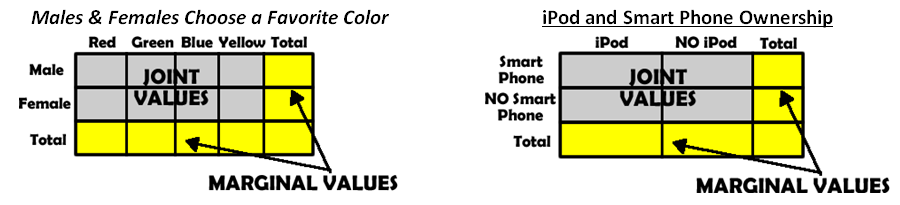
So far we have used lists, tree diagrams, and Venn diagrams to organize our data and determine our probabilities. These ways of organizing help us to visualize the probabilities found in the data. Another powerful way of organizing data is to create a two way frequency table. A two way frequency table works when there are two different categories of data. The data from one sample group is shown as it relates to two different categories. One Category is represented by the rows of the table and the other category is represented by the columns. Entries in the "Total" row and "Total" column are called marginal frequencies. A way to remember this is that the margins of a page are around the perimeter of the page and marginal frequencies are around the edge of the table. Entries in the body of the table are called joint frequencies. A way to remember this is that these values are shared by a column and a row and so they are jointly used by both categories. Below are examples of two way frequency tables.
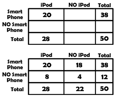
Let us look at an example - a group of 50 students were asked about iPod and Smart phone ownership, 28 owned an iPod, 38 owned a smart phone, and 20 owned both.
The number students surveyed represents the sample space and so it is the total of both the row and column marginal values. The other values can be entered in their locations. From these values we can begin to fill in the rest of the two way table.
By organizing things in a two way table we are able to determine a number of other relationships using simple addition and subtraction. For example we can determine that there would be 18 students that have a smart phone but not an iPod because 38 – 20 = 18 or that 8 students have an iPod but not a Smart Phone because 28 – 20 = 8. |
 |
CONCEPT 2 – Basic Probabilities in Two Way Frequency Tables
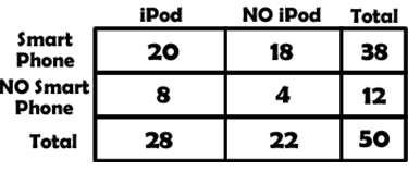
From the two way table many basic probabilities can be calculated. The marginal values provide us the probabilities of each event occurring and in some cases their complements.
BASIC PROBABILITIES
P(iPod) = 28/50 P(Smart Phone) = 38/50
P(Not iPod) = 22/50 P(Not Smart Phone) = 12/50 |
 |
CONCEPT 3 – The Intersection, “AND”, in Two Way Frequency Tables
COMPOUND PROBABILITIES – Intersection
The intersection is found at the intersection of the row and column. Thus P(Smart Phone and iPod) is found at the intersection of the Smart Phone row and the iPod column.
P(Smart Phone and iPod) = 20/50
P(No Smart Phone and No iPod) = 4/50
P(No Smart Phone and iPod) = 8/50 |
 |
CONCEPT 4 – The Union, “OR”, in Two Way Frequency Tables
The union is not as easy to find in the two way table as the intersection. Many students think that the P(Smart Phone or iPod) is simply the addition of the P(Smart Phone) and the P(iPod). This is not the correct way to calculate it because the intersection value gets double counted.
P(Smart Phone or iPod) = 46/50
P(No Smart Phone or No iPod) = 30/50 |
 |
CONCEPT 5 – Conditional Probabilities in Two Way Frequency Tables
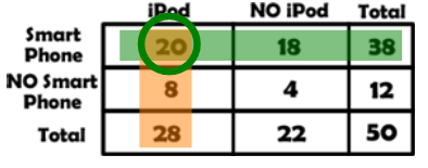
The phrase GIVEN THAT alters the sample space. Given that narrows down the total number of outcomes to a single row or column
.
CONDITIONAL PROBABILITIES
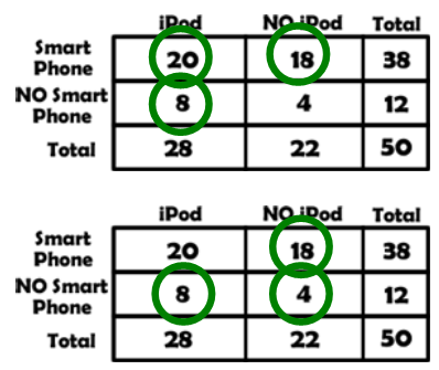
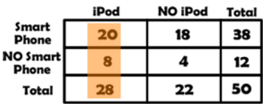
P(Smart Phone|iPod) = 20/28
P(No Smart Phone|iPod) = 8/28
Because we know that they have an iPod we can look at the conditional probabilities for that column. |
 |
CONDITIONAL PROBABILITIES
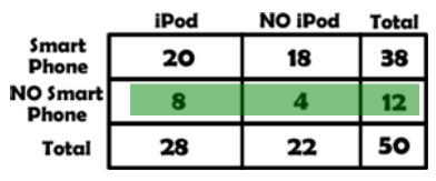
P(iPod|No Smart Phone) = 8/12
P(No iPod|No Smart Phone) = 4/12
Because we know that they don’t have a Smart Phone we can look at the conditional probabilities for that row. |
 |
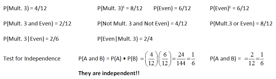
CONCEPT 6 – Determining Independence in Two Way Tables
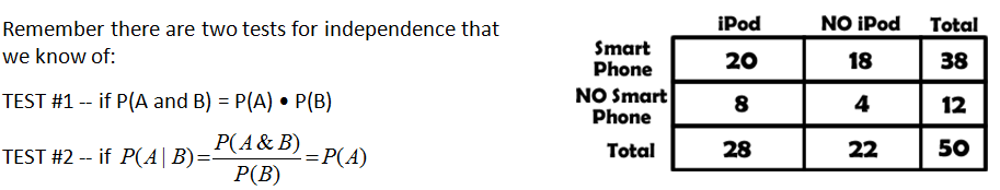
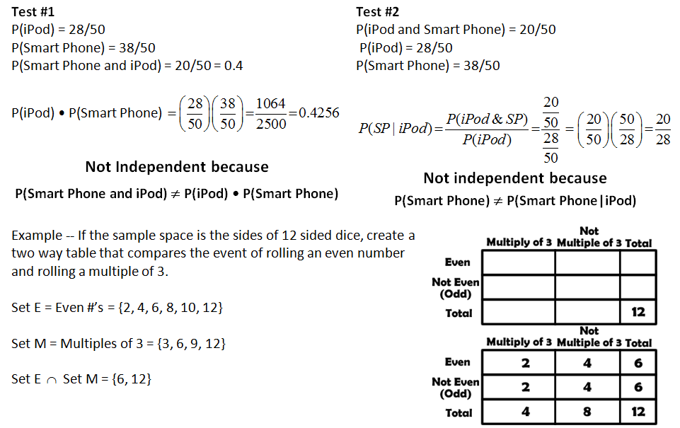
From the chart, determine the probabilities.
CONCEPT 7 – Two Way Relative Frequency Tables
Sometimes instead of the data in the table being actual data counts, like 10 boys or 32 liking swimming, the numbers in the tables have already been converted to their probabilities – their relative frequencies. So the data in the table is not the actual numbers but simply how they RELATE to each other.
Entries in a two way frequency tables are simply tallies or raw data. Probabilities must be calculated using the frequencies.
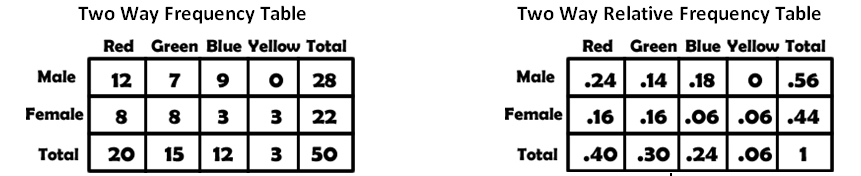
P(Male) = 28/50 P(Female) = 22/50
P(Red) = 20/50 P(Yellow) = 3/50
P(Male and Red) = 12/50
P(Male or Red) = (12 + 7 + 9 + 0 + 8)/50 = 36/50 |
In a two way relative frequency table the data has already been converted to relative frequencies (probabilities). From the table we can find probabilities quickly:
P(Male) = 0.56 P(Female) = 0.44
P(Red) = 0.40 P(Yellow) = 0.06
P(Male and Red) = 0.24
P(Male or Red) = 0.24 + 0.14 + 0.18 + 0.16 = 0.72
Two way relative frequency tables will ALWAYS HAVE 1
as the sum of the row and column marginal values. |
|